Why Sea Floor Density in the Open Ocean is the Key to US East Coast Flood Risk

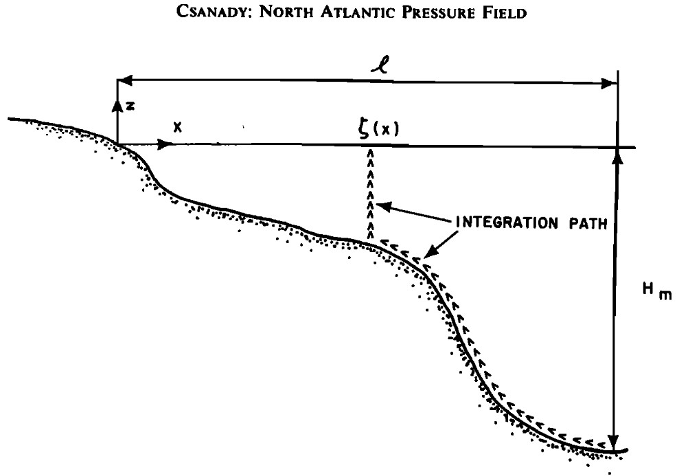
Figure 3 from Csanady (1979). Schematic cross section along a western boundary (x increasing eastward). The arrows identify the paths of density integration used to compute coastal steric setup.

This blog post and the “Deep Dive” podcast, created by Google Notebook, are based on “Steric-Setup Effects on US East Coast Sea-Level Change” by Steinberg et al. (2026).

Steinberg et al. (2026) investigates coastal sea-level variability along the United States East Coast by examining its connection to open-ocean dynamics through a balanced physics framework. By revisiting a classical study of Csanady (1979), the authors evaluate how seafloor topography and density structures influence cross-shore connectivity in high-resolution regional ocean model outputs across thirty-four stations. The findings demonstrate that steric setup—calculated from bottom density anomalies integrated along the seafloor—effectively approximates coastal sea-level changes (Csanady, 1979), though the required offshore distance varies by geographic region. Specifically, locations north of Cape Hatteras exhibit strong shelf influence, whereas southern stations rely more heavily on continental slope variability. Ultimately, this research provides a robust method for linking coastal tide gauge records to larger-scale circulation patterns and can assist in optimizing ocean observing system design.

1. Introduction: The Coastal Disconnect Puzzle

If you stand on a beach in New York or South Carolina and watch the tide come in, it seems natural to assume that local shoreline sea levels directly reflect the massive, slow-moving changes of the open ocean. Yet, for oceanographers, comparing local tide gauge records to deep-ocean sea-level trends has long presented a puzzling disconnect. Why do measurements taken right at the beach frequently fail to align with dynamic sea-level shifts occurring just a few hundred miles offshore?

Part of the answer lies in coastal insulation. While coastal tide gauges provide some of our longest oceanographic records, shoreline waters are continually jostled by local atmospheric forces, coastally trapped waves, boundary currents, and underwater topography (bathymetry). These bathymetric gradients and boundary dynamics create a protective buffer zone, insulating the coast from open-ocean variability.

This creates a fascinating paradox. Recent studies reveal that multi-year sea-level fluctuations along the US East Coast correlate strongly with gyre-scale circulation and heat divergence in the subtropical North Atlantic. Despite these broad statistical links, the exact physical mechanisms bridging coastal waters with open-ocean shifts have remained elusive.

A new study by Steinberg et al. (2026) resolves this puzzle. Using high-resolution regional ocean model output—specifically the Geophysical Fluid Dynamics Laboratory’s NWA12 model ($1/12^\circ$ horizontal resolution with 75 vertical layers, spanning 1993–2022)—researchers evaluated a physics-informed framework across 34 coastal stations ($27^\circ\text{N} to 42^\circ\text{N}$) along the US East Coast. By evaluating sea level, ocean pressure, density, and velocity directly along the ocean bottom, this balanced dynamics framework reveals precisely how coastal waters “feel” open-ocean changes. In particular, the study revisited a classic paper by Csanady (1979) demonstrating that the coastal steric setup is
proportional to an integral of anomalous bottom density up the continental topography.

2. Insight 1: Ocean Bottom Density Acts as a Hidden “Steric Setup” Remote Control

To understand how offshore ocean signals reach the shoreline, oceanographers separate sea-level changes into two fundamental drivers: mass (manometric,$\eta_m$) and density (steric, $\eta_\rho$) contributions.

At monthly and longer timescales, density-driven steric changes dominate deep offshore waters, where warm or fresh water expands the ocean column. Right at the shallow coast, however, sea-level variations primarily reflect local mass changes—driven by wind forcing, atmospheric pressure, or water mass transformations that cause cross-shore mass redistribution.

How does deep-water density expansion translate into shallow coastal mass shifts? The answer lies in steric setup ($\eta_{ss}$). Derived from hydrostatic and geostrophic balances along the seafloor slope, steric setup calculates coastal sea level by integrating ocean bottom density anomalies ($\rho_b$) up the rising underwater topography:

$\eta_{ss} = -\frac{1}{\rho_0} \int_{z=0}^{z=\eta_b} \rho_b \, d\eta_b$

Because there is a direct one-to-one mapping between seafloor depth ($z = \eta_b$) and cross-shore distance (x), integrating bottom density anomalies along the seafloor slope captures how deep density gradients drive near-shore pressure variations.

“This framework provides a link between offshore ocean water mass and circulation changes and sea level changes at the coast through specific consideration of the way in which density and ocean depth increases with distance offshore.”

Instead of needing full-depth water column sampling across vast expanses of open water, measuring bottom density along the seafloor slope allows oceanographers to reconstruct coastal sea level with remarkable physical precision.

3. Insight 2: A Tale of Two Coasts — Cape Hatteras Divides the US East Coast

One of the most striking findings of the study is that cross-shore ocean connectivity is far from uniform. The US East Coast is sharply divided into two distinct dynamical regimes, split neatly by Cape Hatteras:

• North of Cape Hatteras (e.g., New York, NY): Coastal sea level correlates strongly with bottom density variations occurring across the continental shelf (depths under 150 meters). As cross-shore integrals extend across the steadily sloped shelf, model predictive skill increases incrementally and continuously.
• South of Cape Hatteras (e.g., Charleston, SC): Coastal sea level shows almost no connection to bottom density changes across the shallow inner shelf, where water depths remain under 35 meters across distances up to 100 kilometers offshore. Predictive skill remains below 0.25 on the inner shelf and suddenly spikes (>0.75 to 0.90) only when calculations cross the shelf break into the steeper continental slope (depths exceeding 150 meters).

What drives this dramatic regional divergence? Seafloor hypsometry—the distribution of seafloor elevation and cross-shore slope. South of Cape Hatteras, a broad, flat, shallow shelf insulates the shore until reaching the steep continental slope, directly underneath the Gulf Stream axis. North of Cape Hatteras, the shelf slopes more rapidly with distance offshore, allowing shelf-density variations to map directly onto coastal sea level.

4. Insight 3: Depth Rules Over Distance — The Offshore “Hot-Spot” Thresholds

It is easy to assume that the closer an ocean measurement is taken to the beach, the better it will predict coastal flood risks. However, the seafloor framework demonstrates that physical distance from the coast is far less important than water depth.

Predictive skill does not increase linearly with distance offshore. Instead, model skill exhibits sharp threshold jumps once transects cross specific depth milestones—most notably crossing the 150-meter isobath at the shelf break. Evaluating the three right-hand terms of the seafloor balance framework illustrates why:

1. Steric Setup ($\eta_{ss}$): Becomes the dominant predictor once cross-shore integrals reach across the shelf break into deep water. Integrating steric setup across the shelf break leaves a residual variance of less than 25% compared to variance at the coast.
2. Manometric Sea Level ($\eta_m$): Mass contributions explain nearly all variability right at the shallow coast, but rapidly uncouple from manometric changes occurring over deeper open-ocean waters.
3. Bottom Geostrophic Velocity ($\eta_{vb,g}$): Cross-slope bottom currents provide a smaller overall contribution to total skill (typically <0.1). Near Cape Hatteras and strong wind-driven northern zones, velocity terms can suffer skill degradation due to intense Gulf Stream boundary currents, ageostrophic Ekman transport, sub-mesoscale turbulence, and wind forcing.

Pinpointing these exact depth thresholds reveals target “hot-spots” of ocean connectivity, where seafloor density changes exert maximum control over shoreline water levels.

5. Insight 4: Isopycnal Outcropping — How Seafloor Density Relates Coastal Sea Level to the AMOC

Beyond localized pressure balances, the seafloor framework exposes a direct dynamical conduit between coastal tide gauges and large-scale climate engines like the Atlantic Meridional Overturning Circulation (AMOC).

Ocean bottom density anomalies ($\rho_b$) measured along the continental slope correspond to specific ocean density surfaces—known as isopycnals. These constant-density layers intersect the sloped seafloor at specific depth contours and extend offshore into the open ocean, where they eventually outcrop at the sea surface.

Through this physical pathway, surface air-sea fluxes, buoyancy changes, and open-ocean heat content shifts in the North Atlantic alter the density of specific water masses. Because these water masses are bounded by isopycnals that rest against the continental slope, open-ocean overturning signals directly tilt coastal pressure gradients. The seafloor acts as an physical telegraph, translating large-scale AMOC transformations directly into coastal sea-level setup.

6. Insight 5: Smarter Observing Systems — Transforming Climate Readiness

These insights provide a practical blueprint for revolutionizing ocean observing networks and climate adaptation strategies:

• Targeted Sensor Deployment: Instead of deploying costly, exhaustive water-column monitoring across broad ocean basins, observing networks can place targeted ocean bottom temperature, salinity, and pressure sensors at strategic slope hot-spots (e.g., along the 150 m to 800 m isobaths).
• Enhanced Predictive Models: Feeding targeted bottom-density data into regional data-assimilative forecasting models drastically improves predictive skill while reducing operational complexity.

“With a small set of bottom measurements, data assimilative models may gain predictive skill in anticipating and explaining coastal changes.”

By grounding monitoring infrastructure at critical seafloor depth thresholds, oceanographers can deliver earlier, more reliable flood warnings to low-lying coastal communities.

7. Conclusion: Looking Ahead to a Sharper Picture of Coastal Risk

By anchoring ocean circulation theory to seafloor hypsometry, this framework resolves decades of mystery surrounding the disconnect between open-ocean dynamics and coastal tide gauge records. Recognizing how local seafloor shape—such as the contrast between northern sloped shelves and southern broad flats—filters open-ocean signals provides a far clearer picture of regional flood risk.

As climate change alters global ocean density, heat storage, and major boundary currents, understanding where coastal waters couple with the deep ocean is essential for accurate sea-level projections.

A Thought-Provoking Question: As we deploy smarter seafloor-level monitoring systems along our continental slopes, how will these insights transform the way vulnerable coastal towns invest in flood defenses and prepare for tomorrow’s rising seas?

Steinberg, J. M., Griffies, S. M., & Piecuch, C. G. (2026). Steric-setup effects on US East Coast sea-level change. Geophysical Research Letters, 53, e2026GL124322. https://doi.org/10.1029/2026GL124322

Csanady, G. (1979). The pressure field along the western margin of the North Atlantic. Journal of Geophysical Research, 84(C8), 4905–4915. https://doi.org/10.1029/JC084iC08p04905