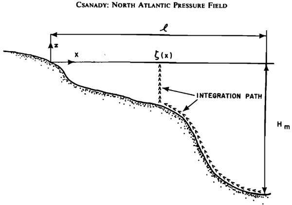
Figure 3 from Csanady (1979). Schematic cross section along a western boundary (x increasing eastward). The arrows identify the paths of density integration used to compute coastal steric setup. This blog post and the “Deep Dive” podcast, created by Google Notebook, are based on “Steric-Setup Effects on US East Coast Sea-Level Change” by Steinberg et... Continue Reading →
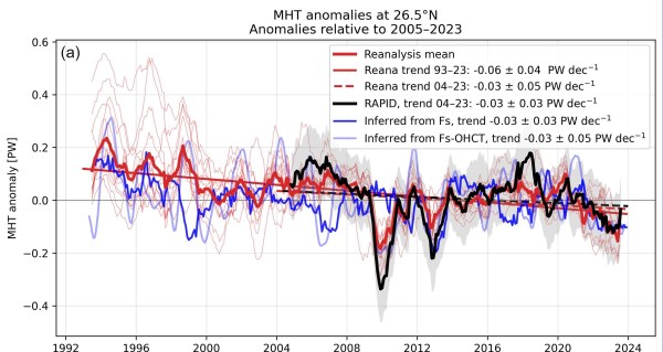
Assessment of 17 Global Ocean Reanalyses Indicates a Widespread Reduction in the AMOC Heat Transport Since the Early 1990s
Figure 11a from Winkelbauer et al. (2026). MHT anomalies at 26.5°N. Thin red curves show individual reanalysis products and the thick red curve denotes the ensemble mean. Thick black curves show RAPID observations. The blue curve in the upper panel shows the inferred MHT estimate, calculated as the mean over ERA5, JRA3Q and MERRA2. the... Continue Reading →
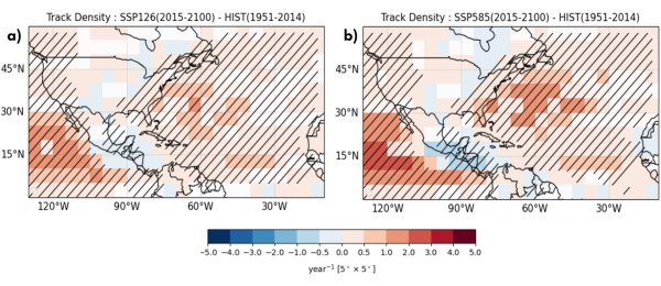
Future Tropical Cyclone Risk in the Gulf Drops while the Southeast Braces for Impact
Figure 1 from Lele et al. (2026). Multi-Model Mean of track density change in the North Atlantic, calculated between future and historical periods for SSP1-2.6 (a) and SSP5-8.5 (b). Stippling shows regions with statistically significant differences at p=0.05 based on a two-sided Student's t-test from the 12-model, 10-track ensemble and 40-intensity ensemble. This blog post... Continue Reading →
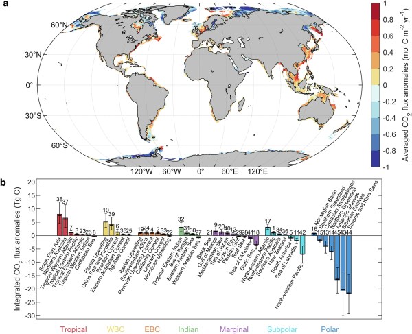
Why High-Latitude Marine Heatwaves are Supercharging Coastal Carbon Sinks
Figure 1 from Hu et al. (2026). a Spatial distribution of averaged air–sea CO2 flux anomalies (mol C m−2 yr−1) during MHW months across the global coastal ocean, derived from the observation-based ULB–SOM–FFN–coastalv2 dataset. Positive anomalies indicate enhanced CO2 outgassing or reduced uptake, whereas negative anomalies represent enhanced uptake or reduced outgassing. b Integrated CO2 flux anomalies (Tg C) across 45 coastal... Continue Reading →
Why the Pacific is Cooling in a Warming World
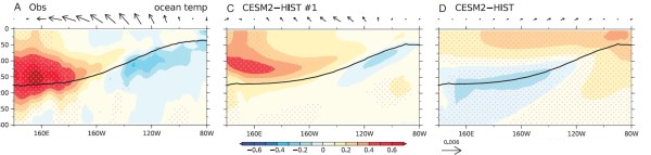
Derived from Figure 2 in Xie et al. (2026). Observed and simulated 1982–2024 trends in equatorial ocean temperature. Linear trend of equatorial (2.5°S to 2.5°N mean) ocean temperature trends (°C/decade) in (A) OISST, (C) a CESM2-HIST member run with the strongest La Nina-like trend, and (D) the CESM2-HIST ensemble mean. Stippling indicates 90% confidence. The... Continue Reading →
Is the Indian Ocean Flooding the U.S. East Coast?
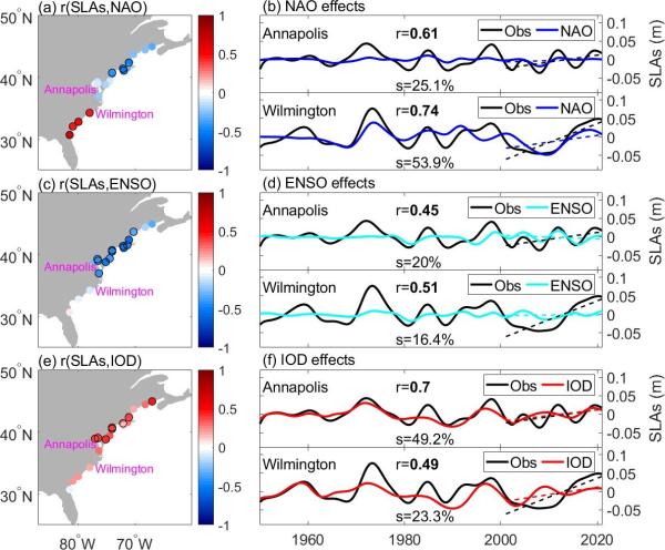
Figure 5 from Zhu et al. (2026). Relationships between decadal sea level anomalies (SLAs) and climate modes for the 1950-2020 period. (a) Correlation coefficients between decadal SLAs (with global mean sea level (GMSL) removed) from tide gauge data and the North Atlantic Oscillation (NAO) index. (b) Decadal SLAs from tide gauge observation (black line) and... Continue Reading →
Why the South Atlantic is Getting Saltier and Why It Matters for Our Climate
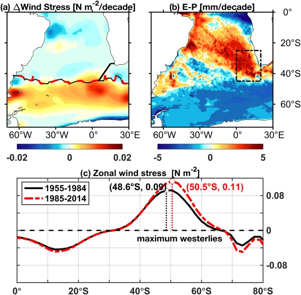
Figure 6 from Cui et al. (2026): (a) Linear trend of zonal wind stress (units: N m−2/decade) averaged over the period 1955–2014 from ERA5. The black solid line indicates the position of the Subtropical Front (STF) during 1955–1984, while the red dashed line represents the STF position during 1985–2014. The black polyline marks the location of... Continue Reading →
Is Global Warming Changing the Pacific Ocean’s Natural Cycles?
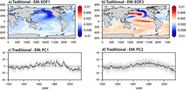
Figure 4 from Xing et al. (2025): Differences between the traditional and ensemble-mean removed methods (hereafter traditional-EM). (a) EOF1 and (b)) EOF2 spatial pattern; here differences are calculated between the ensemble mean of the traditional method applied to each ensemble member, and the ensemble mean of PDV calculated using the ensemble mean removed method. All calculations... Continue Reading →
SST Anomalies in the Tropical Eastern Pacific can dictate the climate of the North Atlantic a decade later
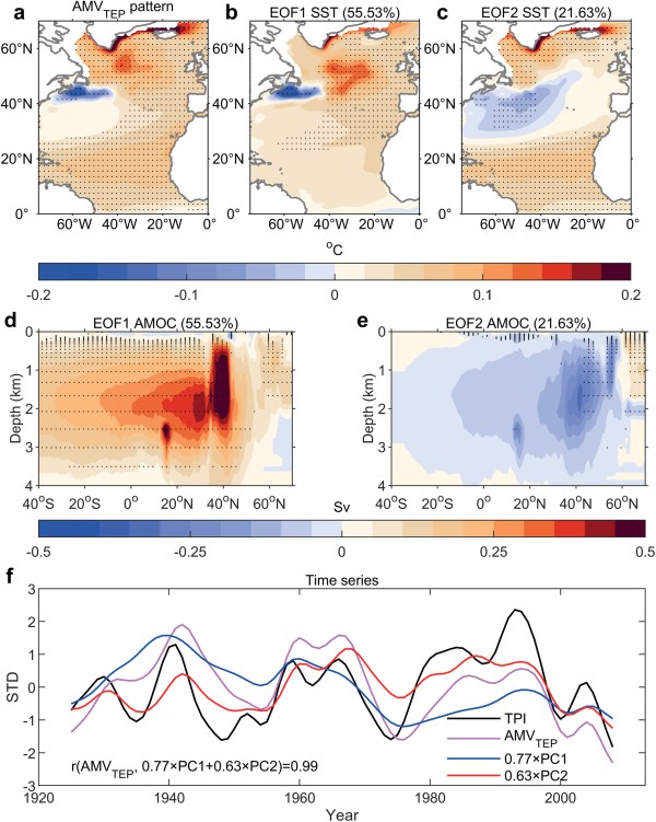
Figure 1 from Yang et al. (2026): The two leading joint EOF modes and their PCs of North Atlantic SST and AMOC decadal variability. (a) Decadal SST anomalies regressed onto the AMVTEP. Decadal SST (b) and AMOC (d) anomalies regressed onto the PC1. In panels (c, e) Same as (b, d) but for the PC2. Stipplings in (a–e) denote... Continue Reading →
New Study Reveals Key Local Blind Spots in Climate Model Projections
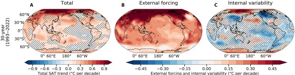
Fig. 2 from Aru et al. (2026): Partitioning of observed SAT trend patterns into external forcing and internal variability. (A) Total, (B) external forcing, and (C) internal variability observed SAT trend patterns for the most recent (D to F) 30-year (1993–2022) periods, respectively, by regressing observed local anomalies against the 1850–2022 MMLE GSAT time series. Hatched regions... Continue Reading →