
For several years, I have been trying to find time and energy to learn GFDL’s Modular Ocean Model version 6 (MOM6), and Python program language. Finally, I have the time and energy to do so. However, I don’t have High Performance Computing resources available to me. So, I had no choice but to work on my Chromebook Plus laptop, which is the only personal computer that works without crashing every 5 min. My Chromebook Plus laptop is equipped with Intel Core i3-N305 processors with 8 cores, 8 GB of memory and 451 GB of solid state drive. I paid $307.97 ($329.53 including sales tax) when I bought it from Amazon about a year ago when it was on sale.
First, I had to activate the Linux development environment to use “Crostini” OS, which is Linux on Chrom OS. I had to install many basic Linux libraries, such as “visual studio code” for code editing, “GNU nano” (a command line text editor similar to emacs, but much simpler), PMEL’s “ferret” for a quick look at model output, “atrill” for opening ps graphic files, “nco” and “cdo” for handling netcdf files. Of course, I also installed Python, “miniconda” for python library installation and management, and numerous Python libraries such as “matplotlib” for plotting, “numPy” for mathematical computing, and “cartopy” for geographic map related processing, one by one as needed.
It took some time for me to understand the concept of creating and activating “env” for different Python projects. I understand that it is necessary to avoid any conflict in using different versions of libraries for different project. But, it is still very annoying to install the same package multiple times for different projects, although I am slowly adjusting to this practice in Python coding.
I mainly followed GFDL’s MOM6-example wiki in github to install MOM6 on my Chromebook. This wiki page provides a step-by-step guide to install and run MOM6, including how to install gfortran, an open source fortran compiler, and openMPI, an open source library for parallel computing. Thanks to the amazing MOM6 tutorial, I was able to install MOM6 and carry out a test run in a day. First, I was able to run an ocean-only global ocean example case (at 1×1 degree resolution) using my 8 CPU cores. But, it was too slow. So, I switched to an ocean-ice coupled Baltic sea example case (at 0.5 x 0.5 degree resolution). I could run this example case with only 4 CPU cores. It took only a couple of hours to run it for one full year. I spent some time to fine tune my running script. My colleague, Dongmin Kim, kindly helped me to prepare a running script that automatically restart MOM6 after each run to run the model for multiple years. It took many days of trial and error to debug and fine tune the script. But, I think it is more or less working now.
After learning MOM6 codes and scripts for the hybrid, layer, and z-star vertical coordinate, I decided to set up a new model domain for the Atlantic Ocean because my main interest is to simulate the Atlantic Meridional Overturning Circulation (AMOC) using MOM6. I got some help from my colleague, Fabian Gomez who did configure a new model domain for the West Florida Shelf using MOM6. Basically, I created a sub-domain for the Atlantic Ocean from an ocean-ice global ocean (at 1×1 degree resolution) example case. I used the MOM6 sponge layer routine to prescribe the damping around the northern (at around 70N) and southern boundaries (at 20S), and the area between the Mediterranean Sea and the Atlantic Ocean at the damping time between 20 to 90 days. I was able to run the Atlantic domain case (116 x 157 grid points) for one year in about 3 ~ 4 hours using all 8 CPU cores.
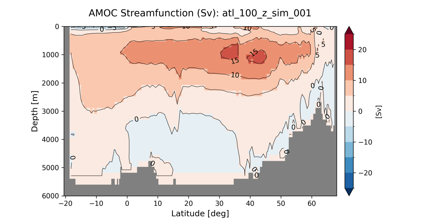
Then, I followed MOM6 analysis cookbook to draw some basic figures using python routines. Ultimately, I was able to compute the AMOC in depth coordinate (Figure) using xoverturning python library. I had to change some of the xoverturning python codes to bypass some technical issues that involve coordinate attribute and the periodic domain. My next goal is carry out a robust diagnostic simulation by nudging the model temperature (T) and salinity (S) of the entire model domain toward observations using World Ocean Atlas 23, and then compare the AMOC with and without the T & S nudging. More to come later.
Figure. Time-averaged AMOC for the year-3 in depth coordinate derived from the Atlantic domain MOM6 run at 1×1 degree resolution, and with 50 z-star coordinate layers. The simulation was carried out on Acer Chromebook plus 514 (Intel Core i3-N305 processors with 8 cores, 8 GB of memory and 451 GB of solid state drive). It took about 4 hours to complete the one full year simulation.

Leave a comment